Processor In The Loop
Once you are convinced your autocoded embedded jMPC controller is working correctly on the development machine, by running the testbenches, the next step is to ensure the controller works on the desired embedded target. To assist with this process, the toolbox automatically generates jMPC_pil.c which contains routines for communicating between an embedded jMPC controller on an embedded target, and the jMPC Toolbox running on a development machine via Serial/UART, in the following manner:
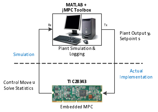
In the above figure the TI C28343 is a reference embedded platform used within my Ph.D. work, but can be substituted by any embedded processor with an FPU, appropriate RAM and a serial interface.
Required User Functions
In order to use the PIL functionality, the user must implement four simple routines on their embedded device:
-
void serial_tx(ucharT a)Transmit a byte over the serial interface.
-
ucharT serial_rx(void)Receive a byte over the serial interface.
-
void timer_start(void)Start a microsecond timer.
-
ulongT timer_stop(void)Stop the microsecond timer, return elapsed microseconds as an unsigned long.
From this point, the "main" function of the embedded application can be as simple as:
void main(void)
{
   // Setup processor
   setup();

   // Enter PIL Mode
   PILSim();
}
Where the while(1) is handled within the call to PILSim(). Note nothing fancy (DMA/interrupt driven) is required for the serial interface as the entire application is effectively sequential. Additionally the timer routine can just return 0 if no benchmark of timing is required.
The above application is compiled with the autogenerated embedded jMPC source files and loaded onto the embedded target and run. It will sit waiting for the development machine to start the simulation.
jMPC PIL Simulation
With the embedded MPC controller loaded on the embedded target, it requires a plant to "control". To automate this process, the toolbox comes with a PIL simulation mode. In this mode, the plant dynamics are simulated in MATLAB, and the controller is run on the embedded target. The plant output and setpoint is sent to the embedded device, the embedded device completes the MPC control calculation, and then sends back the control input (together with solver statistics).
Following the first example in Examples/PIL_Example.m, the only changes required are to tell the toolbox which serial port to use (obviously match to your USB Serial adapator COM port, plus baudrate as configured on the embedded target):
simopts.opts.serialdevice = serial('COM6','BaudRate',1250000);
and change the simulation mode to 'PIL' and the toolbox will handle the rest!
simpil = sim(MPC1,simopts,'pil')
The same plots are available from a PIL simulation, so summary, detail and timing information can be plotted:
plot(MPC1,simpil,'timing');
Additionally, if you wish to verify the results against a development PC jMPC simulation, simply run it locally and use compare to compare simulation results.
simMX = sim(MPC1,simopts,'mex');
compare(MPC1,simMX, simpil);