Embedded MPC Control of a 3DOF Helicopter
To demonstrate control of a real system using the jMPC Toolbox, the Quanser 3DOF Helicopter lab system was used together with custom Data Acquisition (DAQ) hardware and a TI C2000 Evaluation Kit. The system is connected as below, with the embedded target in the bottom right, custom DAQ in the bottom center, and the 3DOF Helicopter and associated power amplifier in the center:
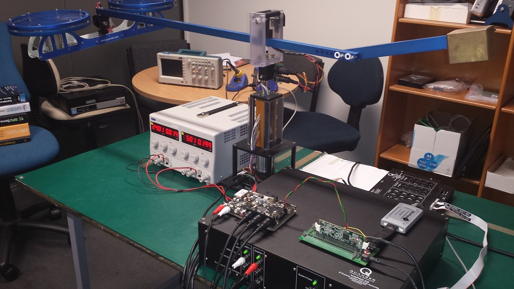
The custom DAQ allowed a simple serial interface to be developed between the Quanser lab equipment and any embedded device, removing the need for the embedded target to also provide quadrature inputs, ADCs, DACs, etc.
MATLAB Setup
The toolbox comes with the files necessary to recreate this setup in Examples/Quanser 3DOF Helicopter. This is copied below for reference from main_Q3DOF.m:
%Get Nonlinear and Linear Models + Parameters
[Gs, Vop, nlheli, param] = setup_embed_heli();
%Convert Linear Model to Discrete
Ts = 0.03; %30ms
Model = jSS(c2d(Gs,Ts));
%MPC Model
x_op = zeros(6,1);
Model = Model.SetLinearization(Vop,x_op);
Model.x0 = x_op;

%Build Plant Model
Plant = jNL(nlheli,Model.C,param);

%Horizons & Time
Np = 80;
Nc = [5 5];
T = 1200;
%Setpoint (Elevation, Pitch, Rotation)
setp = zeros(T,2);
setp(50:end,1) = 0.2618;
setp(300:end,2) = 1.5472;
setp(800:end,2) = -1.0472;
%Constraints
con=[]; pitch = 30*pi/180;
con.u = [-20 20 Inf;
         -20 20 Inf];
con.y = [-Inf   Inf;
         -pitch pitch;
         -Inf   Inf];
con.slack = [Inf 1000 Inf];

%Weights
uwt = [1 1]';
ywt = [12 0 5]'; %[elev pit rot]
%Estimator Gain
Q = 2*eye(6); R = 0.1*eye(3); Q(4,4) = 1; Q(5,5) = 1; Q(6,6) = 0.1;
Kest = dlqe(Model,Q,R);

%Single precision, lower QP tol for speed and set initial control at
%linearization point
opts = jMPCset('Single',1,'QPTol',1e-4,'InitialU',Vop);

%-- Build MPC & Simulation --%
MPC1 = jMPC(Model,Np,Nc,uwt,ywt,con,Kest,opts)
simopts = jSIM(MPC1,Plant,T,setp);
%Add serial port connected to 3-DOF acquisition system
sd = serial('COM6','BaudRate',1250000);
simopts.opts.serialdevice = sd;

%-- Simulate & Plot Result --%
simresult = sim(MPC1,simopts)
plot(MPC1,simresult,'timing');
A few core observations from the above script:
- The sampling frequency has been set as 33.33Hz. This is a little slower than we would normally like for the dynamics of this system, but is sufficient for this problem.
- The prediction horizon has been set as 80 samples, or 2.4 seconds. Again, lower than we would like, but sufficient.
- The control blocking moves were hand optimized for this problem.
- Constraints are placed on output pitch, but are penalized via a slack term, so they may be exceeded in order to remain feasible.
- There is no control of the output pitch, only a constraint.
- The estimator has been designed based on the noise present in the real system.
- The controller is to be run (and generated) in single precision.
- The QP tolerance has been relaxed to avoid numerical issues present with reduced precision.
This produces the following plot:
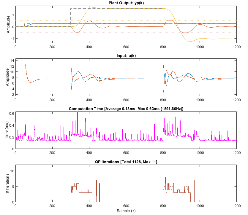
Indicating the controller and tuning is working sufficiently well to move to implementation.
Code Generation
The embedded controller for the above setup is generated using:
eopts = jMPCeset('arch','c2000','dir','..\..\..\Testing\EmbedMPC\');
embed(MPC1,simopts,eopts);
where optionally the output directory can be set to generate the controller source files directly into an embedded IDE project directory. For this problem, the toolbox estimates 42.6KB of memory will be required to store the controller data.
PIL Verification
Prior to actually running the controller with the Quanser hardware, a PIL simulation should be undertaken to ensure the generated controller performs as expected on the target, and at the sampling rate required:
simhelipil = sim(MPC1,simopts,'PIL')
plot(MPC1,simhelipil,'timing');
This produces the following result:
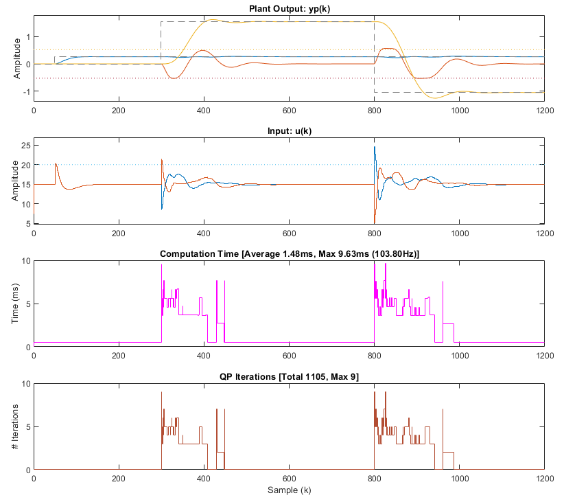
Showing the embedded platform is performing (visually, only) the correction simulation, and the controller is not taking too long to compute the control inputs (worst case 9.6ms of the allocated 30ms). To ensure the control calculation is correct, compare is used:
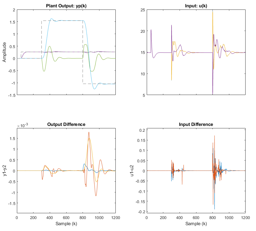
Which shows the results are very similar (differences are expected due to different compilers, optimizations, etc).
Embedded jMPC Control
Running on the embedded target is the generated jMPC controller, together with a simple application that uses a timer interrupt to trigger the control loop. The basic flow is as follows:
- Initialize the processor peripherals
- Wait for the "Start Byte" from the development PC (arbitrary byte to start the controller)
- On each timer interrupt:
- Read the quadrature encoders for the current pitch, elevation and rotation angles from the DAQ
- Pass the angles to the MPC controller and compute the control inputs
- Send the desired motor voltages to the DAQ
- Transmit debug data to the development PC
- Repeat this inner loop
A simple MATLAB script then executes to initiate the controller, and collect the runtime debug data. An example is found in main_Q3DOF.m. The collected debug data can then be plotted as the user likes to examine performance, such as below:
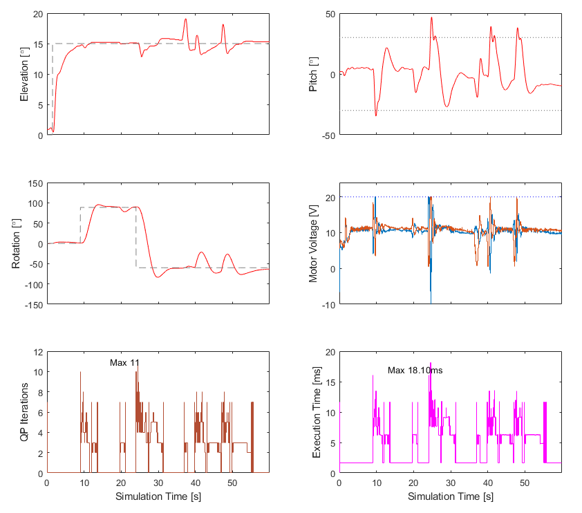
In the above plot, the implementation run included several "Unmeasured Disturbances" (me pushing/disturbing the helicopter) to see how the system reacted. A video of this controller running which produced the above dataset is available on YouTube here.
For more information on this implementation, see Chapter 4 of my thesis.