Continuously Stirred Reactor Controller
jMPC Reference: Examples/Documentation Examples/CSTR_Example.m
Problem Reference: Henson, M. and Seborg, D., Nonlinear Process Control, Prentice Hall PTR, 1997
Nonlinear System Model
The continuous time, ordinary differential equations of the CSTR model are as follows:
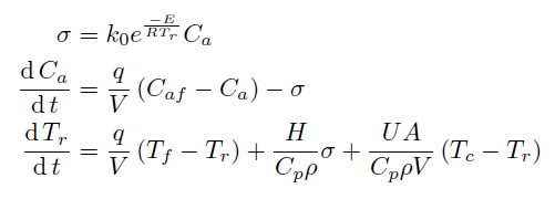
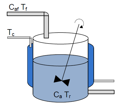
The equations represent a continuously stirred tank reactor with a single reaction from A -> B, and a complete mass and energy balance.
We have defined the state vector, x, as:
| x1 | Concentration of A in reactor (Ca) | [mol/m3] |
| x2 | Temperature of Reactor (Tr) | [K] |
and the output vector, y, as:
| y1 | Concentration of A in reactor (Ca) | [mol/m3] |
| y2 | Temperature of Reactor (Tr) | [K] |
and input, u, as:
| u1 | Concentration of A in feed (Caf) (Measured Disturbance) | [mol/m3] |
| u2 | Temperature of feed (Tf) (Measured Disturbance) | [K] |
| u3 | Temperature of cooling jacket (Tc) | [K] |
Control Objectives
The control objective is to control the temperature of the reactor by adjusting the temperature of the cooling jacket. Both the concentration and temperature of the feed are measured disturbances, and cannot be modified by the controller. The reactor concentration is constrained but not controlled to a setpoint.
System Constraints
The jacket cooling temperature is set as:
And the reactor is constrained as:
Linear MPC with Nonlinear Simulation
Step 1 - Build Nonlinear ODE Callback Function
As detailed in creating a jNL object, the first step is to write an m-file which contains the above expressions, suitable for use with a MATLAB integrator:
function xdot = nl_cstr(t,x,u,param)
% Nonlinear CSTR model

%Assign Parameters
[q,V,k0,E,R,H,Cp,rho,UA] = param{:};

r = k0*exp(-E/(R*x(2)))*x(1);

xdot(1,1) = q/V*(u(1)-x(1)) - r;
xdot(2,1) = q/V*(u(2)-x(2)) + (H/(Cp*rho))*r + (UA)/(Cp*rho*V)*(u(3)-x(2));

end
The file, nl_cstr.m, is saved in a suitable folder on the MATLAB path.
Step 2 - Build the jNL Object
The next step is to build the jNL object, passing the function above as a function handle:
%Parameters
q = 100;     % Volumetric flow rate [m^3/min]
V = 100;     % Volume in reactor [m^3]
k0 = 7.2e10; % Pre-exponential nonthermal factor [1/min]
E = 7.2752e4;% Activation energy in the Arrhenius Equation [J/mol]
R = 8.31451; % Universal Gas Constant [J/mol-K]
H = 5e4;     % Heat of Reaction [J/mol]
Cp = .239;   % Heat capacity (J/g-K)
rho = 1000;  % Density (g/m^3)
UA = 5e4;    % Heat Transfer * Area [J/min-K]

%Output Matrix
C = eye(2);

%Nonlinear Plant
param = {q,V,k0,E,R,H,Cp,rho,UA};  %parameter cell array
Plant = jNL(@nl_cstr,C,param);
Note we have passed the parameters as a cell array, and also retained the linear C output matrix for now. This could also be a function handle to a nonlinear output function.
Step 3 - Linearize the jNL Object
In order to use the nonlinear plant with our linear MPC controller, we must linearize the ODE function and generate the required linear state space model. The system is linearized about an unsteady operating point as specified in the original reference:
%Initial U
CAf = 1; % Feed Concentration [mol/m^3]
Tf = 350; % Feed Temperature [K]
Tc = 300; % Coolant Temperature [K]

%Linearize Plant
u0 = [CAf Tf Tc]';
xop = [0.5 350]'; %unstable operating point [Ca Tr]
Model = linearize(Plant,u0,xop,'ode15s');
Note in this instance we have specified to use ode15s for linearization. While this is not used in this particular scenario (we are not solving for a steady state here), it will be used for all future simulations of this jNL plant (instead of the default ode45).
Step 4 - Create Controller Model
Returned from linearize is a MATLAB lti object containing the linearized model of our system. This must be converted to a jSS object, and discretized to be used to build an MPC controller:
%Build jSS object & discretize
Model = jSS(Model);
Ts = 0.05;
Model = c2d(Model,Ts)
In order to assign the measured disturbances in the model, we use the following method:
%Set Measured Disturbances (Caf,Tf)
Model = SetMeasuredDist(Model,[1 2]); %Provide index of which inputs are mdist
Step 5 - Setup MPC Specifications
The MPC controller is specified as follows:
%Horizons
Np = 30;          %Prediction Horizon
Nc = [10 10 10];  %Blocking Moves

%Constraints
con.u = [278.15 450 20];
con.y = [0      3;
         278.15 450];

%Weighting
uwt = 1;
ywt = [0 5]';

%Estimator Gain
Kest = dlqe(Model);
Step 6 - Setup Simulation Options
Next we must setup the simulation environment for our controller:
%Simulation Length
T = 350;

%Setpoint (CA)
setp = zeros(T,1);
setp(:,1) = xop(2);
setp(50:end,1) = xop(2)+25;
setp(200:end,1) = xop(2)-25;

%Measured Disturbances (Caf Tf)
mdist = zeros(T,2); mdist(:,1) = CAf; mdist(:,2) = Tf;
mdist(130:140,1) = CAf+0.1;              %Step disturbance of Caf
mdist(220:260,2) = Tf-linspace(0,20,41); %Slow cooling of Tf
mdist(261:end,2) = Tf-20;                %Tf final

%Set Initial values at linearization point
Plant.x0 = xop;
Model.x0 = xop;
Step 7 - MPC Options
For advanced settings of the MPC controller we use the jMPCset function to create the required options structure. For this example we wish to set the plot titles and axis, as well as setting the initial control input (at k = 0) to the linearization point:
%Set Options
opts = jMPCset('InitialU',u0,...  %Set initial control input at linearization point
               'InputNames',{'Feed Concentration','Feed Temperature','Jacket Temperature'},...
               'InputUnits',{'mol/m^3','K','K'},...
               'OutputNames',{'Reactor Concentration','Reactor Temperature'},...
               'OutputUnits',{'mol/m^3','K'});
Step 8 - Build the MPC Controller & Simulation Options
Now we have specified all we need to build an MPC controller and Simulation environment, we call the two required constructor functions:
%-- Build MPC & Simulation --%
MPC1 = jMPC(Model,Np,Nc,uwt,ywt,con,Kest,opts)
simopts = jSIM(MPC1,Plant,T,setp,[],mdist);
MPC1 is created using the jMPC constructor, where the variables we have declared previously are passed as initialization parameters. simopts is created similarly, except using the jSIM constructor. Both constructors contain appropriate error checking thus the user will be informed of any mistakes when creating either object.
Step 9 - Run the MPC Simulation & Plot Results
With the controller and environment built, we can run the simulation, and plot the results. We use Simulink as the evaluation environment as it runs significantly faster than Matlab for these simulations:
%-- Simulate & Plot Result --%
simresult = sim(MPC1,simopts,'Simulink')
plot(MPC1,simresult,'detail');
The plot produced is shown below:
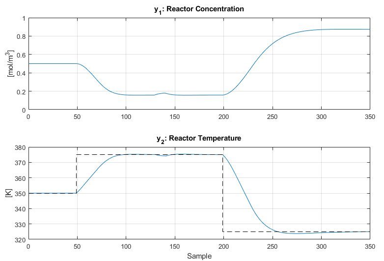
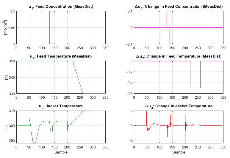
As shown above the system shows good control with minimal overshoot even for large step changes. This particular problem presents a considerable challenge to linear MPC based on the unstable operating point and significant nonlinearities of the system. However correct tuning can give good results, even when responding to disturbances.